News search and recommendation tutorial - embeddings

This is the fourth part of the tutorial series for setting up a Vespa application for personalized news recommendations. The parts are:

1. Getting started
2. A basic news search application - application packages, feeding, query
3. News search - sorting, grouping, and ranking
4. Generating embeddings for users and news articles
5. News recommendation - partial updates (news embeddings), ANNs, filtering
6. News recommendation with searchers - custom searchers, doc processors
7. News recommendation with parent-child - parent-child, tensor ranking
8. Advanced news recommendation - intermission - training a ranking model
9. Advanced news recommendation - ML models

In this part, we'll start transforming our application from news search to recommendation. We won't be using Vespa at all in this part. Our focus is to generate news and user embeddings. We'll start using these embeddings in the next part - you can skip this part if you wish.

The primary function of a recommendation system is to provide items of interest to any given user. The more we know about the user, the better recommendations we can provide. We can view recommendation as search where the query is the user profile. So, in this tutorial we will build upon the previous news search tutorial by creating user profiles and use them to search for relevant news articles.

We start by generating embeddings using a collaborative filtering method. We'll then improve upon that using a content-based approach, which generates embedding based on BERT models. Since we'll use this in a nearest neighbors algorithm, we'll touch upon how the maximum inner product search is transformed to a distance search form.

Let's start with taking a look again at what data the MIND dataset provides for us.

Requirements

We start using some machine learning tools in this tutorial. Specifically, we need Numpy, Scikit-learn, PyTorch, and the HuggingFace Transformers library. Make sure you have all the necessary dependencies by running the following in the sample application directory:

$ python3 -m pip install --ignore-installed -r requirements.txt

The MIND dataset

The MIND dataset, for our purposes in this series of tutorials, consists of two main files: news.tsv and behaviors.tsv. We used the former in the previous tutorial, as that contains all news article content.

The behaviors.tsv file contains a set of impressions. An impression is an ordered list of news articles that was generated for a user. It includes which of those articles the user clicked, and conversely, which ones were not. We designate articles not clicked as "skips". Also included in the impression is a list of articles the user has previously clicked. An example is:

3       U11552  11/11/2019 1:03:52 PM   N2139   N18390-0 N10537-0 N23967-1

Here, user U11552 was shown three articles: N18390, N10537, and N23967, of which the user skipped two and clicked the last one. At that time, the user had previously clicked on article N2139. We can cross-reference with the news.tsv and extract the content of these articles.

We interpret a click as a positive signal for interest and a skip as possibly a negative signal for interest. This is called implicit feedback, as the users haven't explicitly expressed their interests. However, using clicks and skips, we can still start to infer the users' interests.

Collaborative filtering in recommendation systems

A simple approach to provide recommendations to the above would be to extract the categories, subcategories, and/or entities the users have implicitly interacted with, and store these for each user. We can call this a sparse user profile because we store the exact terms of entities or categories. We could then use traditional information retrieval techniques to search for more articles with similar content.

However, by doing this we miss out on a lot of information. For instance, some categories or entities are similar, which could be of interest to the user. Also, users with similar interests tend to click on similar articles. If some type of content was interesting to one user, it would likely be interesting to similar users.

Exploiting this information is called collaborative filtering and the classical approach to this is matrix factorization. In this approach, we create a large matrix with users along one axis and news articles along the other. We'll call this the interaction matrix. Then we factorize this matrix into two smaller matrices, where the product of these two smaller approximates the original.

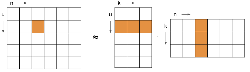
In the image above, you can see a user matrix with as many rows as there are users and a news matrix with as many columns as there are news articles. Each user row, or news column, has the same length, signified by the k dimension. The intuition is that the dot product of the k length vector for a user and news pair approximates the user's interest in the news article. Since the information is compressed into the k length vector, this works across users as well. Thus, the "collaborative" filtering.

These k length vectors can be extracted from the matrices and associated with the user or news article. So, when we want to recommend news articles to a user, we simply find the user's vector and find the articles with the highest dot products. In the following, we will use this approach to generate such embeddings for users and news articles.

Please note, however, this approach would not work well in practice for news recommendation. The reason is that a large part of news recommendation is to recommend new news articles, which might not have received any implicit feedback yet. This is called the "cold start" problem. For such problems, we need to use additional content (often called "side information") of news articles to provide recommendations. We'll tackle this "cold start" a bit later.

Generating embeddings

A standard method for factorizing the interaction matrix is to use Alternating Least Squares. The idea is to randomly fill the user and news matrices and freeze one of the matrices' parameters while solving for the other. By alternating between which matrix is fixed, this can be solved with a traditional least-squares problem. We can iterate the process until convergence.

This tutorial aims to generate embeddings so that the dot product between a user and news vector signifies the probability of a click. Using this signal we can rank news articles by click probability. To train the embedding vectors, we will use a stochastic gradient descent approach to modify the embeddings so that their dot product followed by the logistic function predicts a user click. We use a binary cross-entropy as loss function.

We'll use PyTorch for this. The main PyTorch model class is as follows:

class MF(torch.nn.Module):
    def __init__(self, num_users, num_items, embedding_size):
        super(MF, self).__init__()
        self.user_embeddings = torch.nn.Embedding(num_embeddings=num_users,
                                                  embedding_dim=embedding_size)
        self.news_embeddings = torch.nn.Embedding(num_embeddings=num_items,
                                                  embedding_dim=embedding_size)

    def forward(self, users, items):
        user_embeddings = self.user_embeddings(users)
        news_embeddings = self.news_embeddings(items)
        dot_prod = torch.sum(torch.mul(user_embeddings, news_embeddings), 1)
        return torch.sigmoid(dot_prod)

We use the PyTorch's Embedding class to hold the user and news embeddings. The forward function is the forward pass of the gradient descent. First, the users and items selected for a mini-batch update are extracted from their embedding tables. Then we take the dot-product with a logistic function and return the value. This prediction for user and news pairs is then evaluated against the click or skip labels:

    # forward + backward + optimize
    user_ids, news_ids, labels = batch
    prediction = model(user_ids, news_ids)
    loss = loss_function(prediction.view(-1), labels)
    loss.backward()
    optimizer.step()

This is done across several of epochs. The batch here contains a batch ofuser_ids, news_ids, and labels used for training a mini-batch. For instance, from the example impression above, a training example would be U11552, N23967, 1. The code responsible for generating the training data samples 4 negative examples (skips) for each positive example (click).

The full code can be seen in the sample application, in train_mf.py. Let's go ahead and generate the embeddings:

$ ./src/python/train_mf.py mind 10

This runs the training code for 10 epochs, and deposits the resulting user and news vectors in the mind directory, where the rest of the data is:

Total loss after epoch 1: 573.5299682617188 (3.49713397026062 avg)
Total loss after epoch 2: 551.6585083007812 (3.363771438598633 avg)
...
{'auc': 0.5776, 'mrr': 0.248, 'ndcg@5': 0.2573, 'ndcg@10': 0.317}
{'auc': 0.4988, 'mrr': 0.2154, 'ndcg@5': 0.2182, 'ndcg@10': 0.2824}

We can see the loss reduces over the number of epochs. The two final lines here are ranking metrics run on the training set and validation set. Here, the AUC metric - Area Under the (ROC) Curve - is at 0.5776 for the training set and 0.4988 for the validation set. If you run for a greater number of epochs, you would see the AUC for the training set become much larger than the validation set, around 0.974 and 0.51 respectively if run for 100 epochs.

In this case, the AUC metric measures the probability of ranking relevant news higher than non-relevant news. A score of around 0.5 means that it is totally random. Thus, we haven't learned anything of use for the validation set.

This is not overfitting but rather an instance of the problem mentioned earlier. The validation set contains news articles shown to users a time period after the data in the training set. Thus, most news articles are new, and their embedding vectors are effectively random.

We'll address this next.

Addressing the cold start problem

The approach above based itself on news articles that users interacted with in the training set period. Only the user ids and news article ids were used. To overcome the problem that new articles haven't been seen in the training set, we need to use the article's content features. So, the predictions will be based on the similarity of content a user has previously interacted, rather than the actual news article id.

This is, naturally enough, called content-based recommendation.

The general approach we'll take here is to still rely on a dot product between a user embedding and news embedding, however the news embedding will be constructed from various content features.

The MIND dataset has a few such features we can use. Each news article has a category, a subcategory and zero or more entities extracted from the text. These features are categorical, meaning that they have a finite set of values they can take. To handle these, we'll generate an embedding for each possible value, similar to how we generated embeddings for the user id's and news id's above. These ids are also categorical, after all.

Creating BERT embeddings

However, there are other content features as well such as the title and abstract. To create embeddings from these, we'll employ a BERT-based sentence classifier from the HuggingFace transformers library:

from transformers import BertTokenizer, BertModel
tokenizer = BertTokenizer.from_pretrained('bert-base-uncased')
model = BertModel.from_pretrained('google/bert_uncased_L-8_H-512_A-8')
tokens = tokenizer(title, abstract, return_tensors="pt")
outputs = model(**tokens)
embedding = outputs[0][0][0]

Here, we use a medium-sized BERT model with 8 layers and a hidden dimension size of 512. This means that the embedding will be a vector of size 512. We use the vector from the first CLS token to represent the combined title and abstract.

To generate these embeddings for all news content, run one of the following:

1. Generate embeddings. This might take a while, around an hour for all news articles in the train and dev demo dataset.

   $ python3 src/python/create_bert_embeddings.py mind
   

2. Download pre-processed embeddings:

   $ curl -L -o mind/train/news_embeddings.tsv \
     https://data.vespa.oath.cloud/sample-apps-data/mind_news_embedding.tsv
   $ curl -L -o mind/dev/news_embeddings.tsv \
     https://data.vespa.oath.cloud/sample-apps-data/mind_news_embedding_dev.tsv
   

This creates a news_embeddings.tsv file under the mind/train and mind/dev subdirectories.

Training the model

Now that we have content-based embeddings for each news article, we can train the model to use them. The following figure illustrates the model we are training:

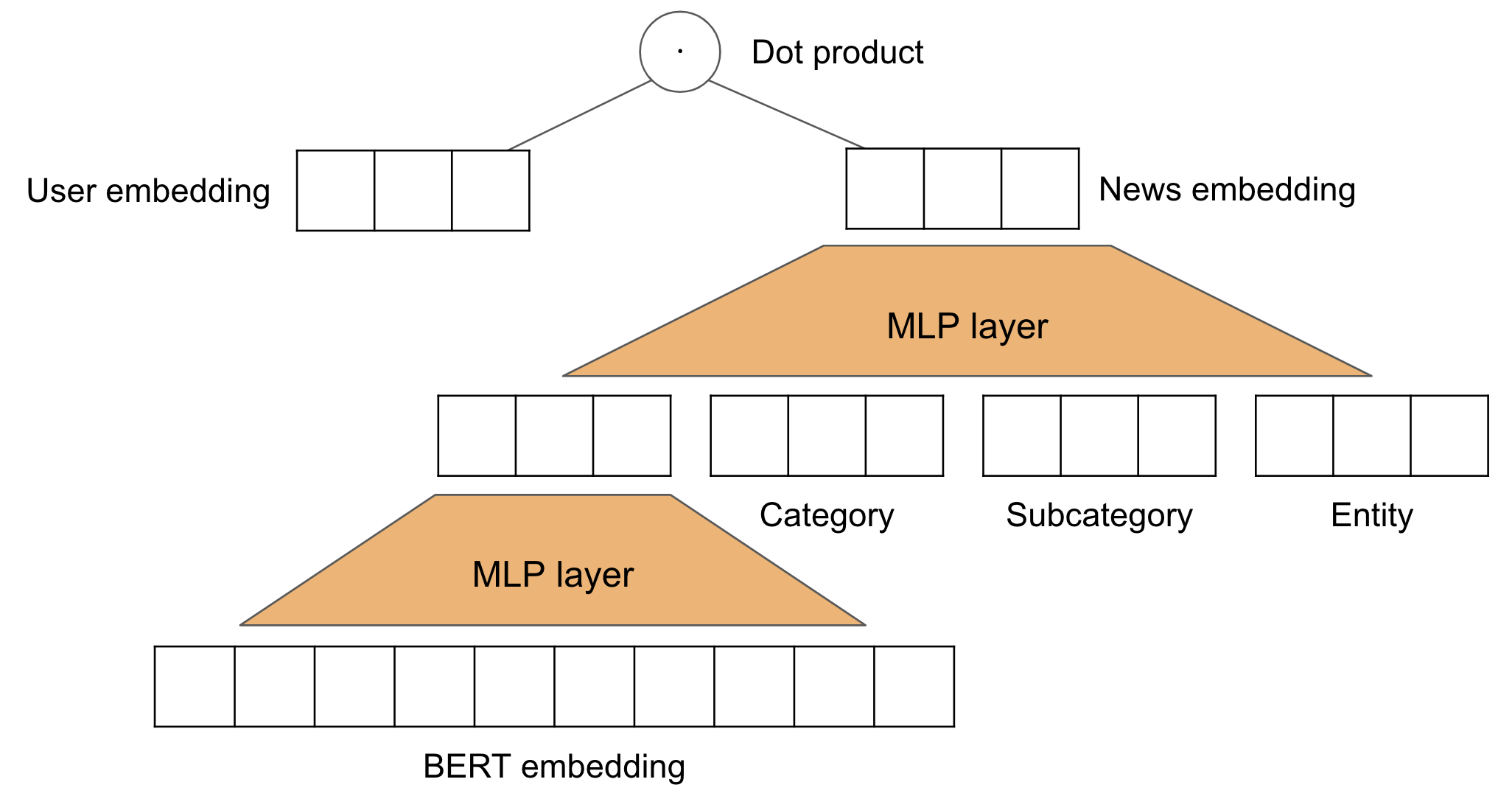
So, we'll pass the 512-dimensional embeddings from the BERT model through a typical neural network layer to reduce dimensions to 50. We then concatenate this representation with the 50 dimensional embeddings for category, subcategory and entity. We only use one entity for now. This representation is then sent through another neural network layer to form the final representation for a news article. Finally, the dot product is taken with the user embedding.

In PyTorch code, this looks like:

class ContentBasedModel(torch.nn.Module):
    def __init__(self,
                 num_users,
                 num_news,
                 num_categories,
                 num_subcategories,
                 num_entities,
                 embedding_size,
                 bert_embeddings):
        super(ContentBasedModel, self).__init__()

        # Embedding tables for category variables
        self.user_embeddings = torch.nn.Embedding(num_embeddings=num_users, embedding_dim=embedding_size)
        self.news_embeddings = torch.nn.Embedding(num_embeddings=num_news, embedding_dim=embedding_size)
        self.cat_embeddings = torch.nn.Embedding(num_embeddings=num_categories, embedding_dim=embedding_size)
        self.sub_cat_embeddings = torch.nn.Embedding(num_embeddings=num_subcategories, embedding_dim=embedding_size)
        self.entity_embeddings = torch.nn.Embedding(num_embeddings=num_entities, embedding_dim=embedding_size)

        # Pretrained BERT embeddings
        self.news_bert_embeddings = torch.nn.Embedding.from_pretrained(bert_embeddings, freeze=True)

        # Linear transformation from BERT size to embedding size (512 -> 50)
        self.news_bert_transform = torch.nn.Linear(bert_embeddings.shape[1], embedding_size)

        # Linear transformation from concatenation of category, subcategory, entity and BERT embedding
        self.news_content_transform = torch.nn.Linear(in_features=embedding_size*5, out_features=embedding_size)

    def get_user_embeddings(self, users):
        return self.user_embeddings(users)

    def get_news_embeddings(self, items, categories, subcategories, entities):
        # Transform BERT representation to a shorter embedding
        bert_embeddings = self.news_bert_embeddings(items)
        bert_embeddings = self.news_bert_transform(bert_embeddings)
        bert_embeddings = torch.sigmoid(bert_embeddings)

        # Create news content representation by concatenating BERT, category, subcategory and entities
        cat_embeddings = self.cat_embeddings(categories)
        news_embeddings = self.news_embeddings(items)
        sub_cat_embeddings = self.sub_cat_embeddings(subcategories)
        entity_embeddings_1 = self.entity_embeddings(entities[:,0])
        news_embedding = torch.cat((news_embeddings, bert_embeddings, cat_embeddings,
                                    sub_cat_embeddings, entity_embeddings_1), 1)
        news_embedding = self.news_content_transform(news_embedding)
        news_embedding = torch.sigmoid(news_embedding)

        return news_embedding

    def forward(self, users, items, categories, subcategories, entities):
        user_embeddings = self.get_user_embeddings(users)
        news_embeddings = self.get_news_embeddings(items, categories, subcategories, entities)
        dot_prod = torch.sum(torch.mul(user_embeddings, news_embeddings), 1)
        return torch.sigmoid(dot_prod)

The forward pass function is pretty much the same as before. You can see the entire training script in train_cold_start.py. Running this results in:

$ python3 src/python/train_cold_start.py mind 10

Total loss after epoch 1: 920.5855102539062 (0.703811526298523 avg)
{'auc': 0.5391, 'mrr': 0.2367, 'ndcg@5': 0.2464, 'ndcg@10': 0.3059}
{'auc': 0.5131, 'mrr': 0.2239, 'ndcg@5': 0.2296, 'ndcg@10': 0.2933}
Total loss after epoch 2: 761.7719116210938 (0.5823944211006165 avg)
{'auc': 0.647, 'mrr': 0.2992, 'ndcg@5': 0.3246, 'ndcg@10': 0.3829}
{'auc': 0.5656, 'mrr': 0.2447, 'ndcg@5': 0.2604, 'ndcg@10': 0.3255}
Total loss after epoch 3: 660.2255859375 (0.5047596096992493 avg)
{'auc': 0.7032, 'mrr': 0.3323, 'ndcg@5': 0.3662, 'ndcg@10': 0.426}
{'auc': 0.5926, 'mrr': 0.2623, 'ndcg@5': 0.285, 'ndcg@10': 0.3474}
Total loss after epoch 4: 625.5714111328125 (0.4782656133174896 avg)
{'auc': 0.7329, 'mrr': 0.3519, 'ndcg@5': 0.3901, 'ndcg@10': 0.4514}
{'auc': 0.5998, 'mrr': 0.2634, 'ndcg@5': 0.2872, 'ndcg@10': 0.3492}
Total loss after epoch 5: 605.7533569335938 (0.4631142020225525 avg)
{'auc': 0.7602, 'mrr': 0.3758, 'ndcg@5': 0.4191, 'ndcg@10': 0.4797}
{'auc': 0.6095, 'mrr': 0.271, 'ndcg@5': 0.2962, 'ndcg@10': 0.358}
Total loss after epoch 6: 588.0604248046875 (0.44958749413490295 avg)
{'auc': 0.7881, 'mrr': 0.3992, 'ndcg@5': 0.4492, 'ndcg@10': 0.5094}
{'auc': 0.6156, 'mrr': 0.2742, 'ndcg@5': 0.3009, 'ndcg@10': 0.3634}
Total loss after epoch 7: 570.162353515625 (0.435903936624527 avg)
{'auc': 0.8141, 'mrr': 0.4268, 'ndcg@5': 0.4837, 'ndcg@10': 0.5408}
{'auc': 0.6201, 'mrr': 0.2777, 'ndcg@5': 0.3044, 'ndcg@10': 0.3676}
Total loss after epoch 8: 551.164306640625 (0.4213794469833374 avg)
{'auc': 0.8382, 'mrr': 0.4546, 'ndcg@5': 0.5184, 'ndcg@10': 0.5734}
{'auc': 0.6223, 'mrr': 0.28, 'ndcg@5': 0.3064, 'ndcg@10': 0.3702}
Total loss after epoch 9: 534.6984252929688 (0.40879085659980774 avg)
{'auc': 0.8577, 'mrr': 0.4785, 'ndcg@5': 0.5479, 'ndcg@10': 0.6009}
{'auc': 0.6266, 'mrr': 0.2847, 'ndcg@5': 0.3115, 'ndcg@10': 0.3747}
Total loss after epoch 10: 517.16748046875 (0.3953879773616791 avg)
{'auc': 0.8758, 'mrr': 0.5074, 'ndcg@5': 0.5818, 'ndcg@10': 0.6316}
{'auc': 0.6249, 'mrr': 0.2842, 'ndcg@5': 0.3114, 'ndcg@10': 0.3733}

This is much better. The AUC score at epoch 9 is a respectable 0.6266. Note that as we train further, the AUC for the dev set starts dropping. This is a sign of overfitting, so we should stop training.

For reference, the baseline model for the MIND competition, Neural News Recommendation with Multi-Head Self-Attention, results in 0.6362. This model additionally uses the user history in each impression to create a better model for the user embedding. For the moment, however, we are satisfied with these, and we'll use them going forward. Feel free to experiment and see if you can achieve better results!

The training script writes these embeddings to the files mind/user_embeddings.tsv and mind/news_embeddings.tsv.

Mapping from inner-product search to euclidean search

These vectors have been trained to maximize the inner product. Finding the best news articles given a user vector is called Maximum Inner Product Search - or MIPS. This form isn't really suitable for efficient retrieval as-is, but it can be mapped to a nearest neighbor search problem, so we can use an efficient approximate nearest neighbors index.

When specifying distance-metric: dotproduct, Vespa uses the technique discussed in Speeding Up the Xbox Recommender System Using a Euclidean Transformation for Inner-Product Spaces to solve the MIPS case. See blog post announcing MIPS support in Vespa.

field embedding type tensor<float>(d0[50]) {
            indexing: attribute | index
            attribute {
                distance-metric: dotproduct
            }
}

See Nearest Neighbor Search for more information on nearest neighbor search and supported distance metrics in Vespa.

We've included a script to create a feed suitable for Vespa:

$ python3 src/python/convert_embeddings_to_vespa_format.py mind

We are now ready to feed these embedding vectors to Vespa.

Conclusion

Now that we've generated user and document embeddings, we can start using these to recommend news items to users. We'll start feeding these in the next part of the tutorial.