Geo Search

To model a geographical position in documents, use a field where the type is position for a single, required position. To allow any number of positions (including none at all) use array<position> instead. This can be used to limit hits (only those documents with a position inside a circular area will be hits), the distance from a point can be used as input to ranking functions, or both.

A geographical point in Vespa is specified using the geographical latitude and longitude. As an example, a location in Sunnyvale, California could be latitude 37.4181488 degrees North, longitude 122.0256157 degrees West. This would be represented as { "lat": 37.4181488, "lng": -122.0256157 } in JSON.

As seen above, positive numbers are used for north (latitudes) and east (longitudes); negative numbers are used for south and west. This is the usual convention.

Sample schema and document

A sample schema could be a business directory, where every business has a position (for its main office or contact point):

schema biz {
    document biz {
        field title type string {
            indexing: index
        }
        field mainloc type position {
            indexing: attribute | summary
        }
    }
    fieldset default {
        fields: title
    }
}

Using this schema is one possible business entry with its location:

{
    "put": "id:mynamespace:biz::business-1",
    "fields": {
        "title":      "Yahoo Inc (main office)",
        "mainloc":    { "lat": 37.4181488, "lng": -122.0256157 }
    }
}

Restrict

The API for adding a geographical restriction is to use a geoLocation clause in the YQL statement, specifying a point and a maximum distance from that point:

$ curl -H "Content-Type: application/json" \
  --data '{"yql" : "select * from sources * where title contains \"office\" and geoLocation(mainloc, 37.416383, -122.024683, \"20 miles\")"}' \
  http://localhost:8080/search/

One can also build or modify the query programmatically by adding a GeoLocationItem anywhere in the query tree.

To use a position for ranking only (without any requirement for a matching position), specify it as a ranking-only term. Use the rank() operation in YQL for this, or a RankItem when building the query programmatically.

At the same time, specify a negative radius (for example -1 m). This matches any position, and computes distance etc. for the closest position in the document. Example:

$ curl -H "Content-Type: application/json" \
  --data '{"yql" : "select * from sources * where rank(title contains \"office\", geoLocation(mainloc, 37.416383, -122.024683, \"-1 m\"))"}' \
  http://localhost:8080/search/

Ranking from a position match

The main rank feature to use for the example above would be distance(mainloc).km and doing further calculation on it, giving better rank to documents that are closer to the wanted (query) position. Here one needs to take into consideration what sort of distances is practical; traveling on foot, by car, or by plane should have quite different ranking scales - using different rank profiles would be one natural way to support that. If the query specifies a maximum distance, that could be sent as an input to ranking as well, and used for scaling.

There is also a closeness(mainloc) which goes from 1.0 at the exact location to 0.0 at a tunable maximum distance, which is enough for many needs.

Useful summary-features

To do further processing, it may be useful to get the computed distance back. The preferred way to do this is to use the associated rank features as summary-features. In particular, distance(fieldname).km gives the geographical distance in kilometers, while distance(fieldname).latitude and distance(fieldname).longitude gives the geographical coordinates for the best location directly, in degrees. These are easy to use programmatically from a searcher, accessing feature values in results for further processing.

Using multiple position fields

For some applications, it can be useful to have several position attributes that may be searched. For example, we could expand the above examples with the locations of subsidiary offices:

schema biz {
    document biz {
        field title type string {
            indexing: index
        }
        field mainloc type position {
            indexing: attribute | summary
        }
        field otherlocs type array<position> {
            indexing: attribute
        }
    }
    fieldset default {
        fields: title
    }
}

Expanding the example business with an office in Australia and one in Norway could look like:

{
    "put": "id:mynamespace:biz::business-1",
    "fields": {
        "title":       "Yahoo Inc (some offices)",
        "mainloc":     { "lat": 37.4, "lng": -122.0 },
        "otherlocs": [ { "lat": -33.9, "lng": 151.2 },
                       { "lat": 63.4, "lng": 10.4 } ]
    }
}

A single query item can only search in one of the position attributes. For a search that spans several fields, use YQL to combine several geoLocation items inside an or clause, or combine several fields into a combined array field (so in the above example, one could duplicate the "mainloc" position into the "otherlocs" array as well, possibly changing the name from "otherlocs" to "all_locs").

Example with airport positions

Distance to path

This example provides an overview of the DistanceToPath rank feature. This feature matches document locations to a path given in the query. Not only does this feature return the closest distance for each document to the path, it also includes the length traveled along the path before reaching the closest point, or intersection. This feature has been nick named the gas feature because of its obvious use case of finding gas stations along a planned trip.

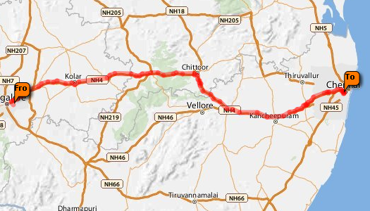
In this example we have been traveling from the US to Bangalore, and we are now planning our trip back. We have decided to rent a car in Bangalore that we are to return upon arrival at the airport in Chennai. We are already quite hungry and wish to stop for a meal once we are outside of town. To avoid having to pay an additional fueling premium, we also wish to refuel just before reaching the airport. We need to figure out what roads to take, what restaurants are available outside of Bangalore, and what fuel stations are available once we get close to Chennai. 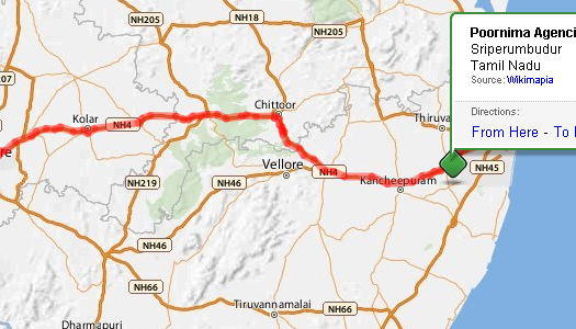Here we have plotted our trip from Bangalore to the airport:

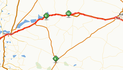
If we search for restaurants along the path, we only see a small subset of all restaurants present in the window of our quite large map. Here you see how the most relevant results are actually all in Bangalore or Chennai:

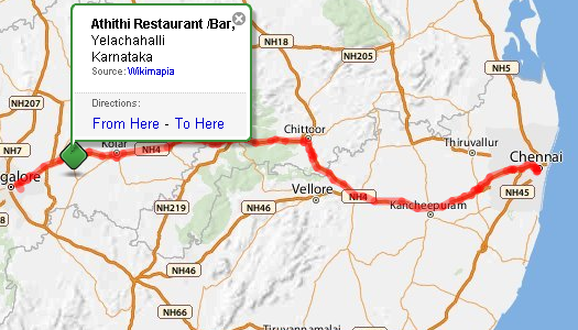
To find the best results, move the map window to just about where we expect to be eating, and redo the search:

This has to be done similarly for finding a gas station near the airport. This illustrates searching for restaurants in a smaller window along the planned trip without DistanceToPath. Next, we outline how DistanceToPath can be used to quickly and easily improve this type of planning to be more convenient for the user.

The nature of this feature requires that the search corpus contains documents with position data. A searcher component needs to be written that is able to pass paths with the queries that lie in the same coordinate space as the searchable documents. Finally, a rank-profile needs to defined that scores documents according to how they match some target distance traveled and at the same time lies close "enough" to the path.

Query Syntax

This document does not describe how to write a searcher plugin for the Container, refer to the container documentation. However, let us review the syntax expected by DistanceToPath. As noted in the the rank features reference, the path is supplied as a query parameter by name of the feature and the path keyword:

yql=(…)&rankproperty.distanceToPath(name).path=(x1,y1,x2,y2,…,xN,yN)

Here name has to match the name of the position attribute that holds the positions data.

The path itself is parsed as a list of N coordinate pairs that together form N-1 line segments:

$$(x_1,y_1) \rightarrow (x_2,y_2), (x_2,y_2) \rightarrow (x_3,y_3), (…), (x_{N-1},y_{N-1}) \rightarrow (x_N,y_N)$$

Rank profile

If we were to disregard our scenario for a few moments, we could suggest the following rank profile:

rank-profile default {
    first-phase {
        expression: nativeRank
    }
    second-phase {
        expression: firstPhase * if (distanceToPath(ll).distance < 10000, 1, 0)
    }
}

This profile will first rank all documents according to Vespa's nativeRank feature, and then do a second pass over the top 100 results and order these based on their distance to our path. If a document lies within 100 metres of our path it retains its relevancy, otherwise its relevancy is set to 0. Such a rank profile would indeed solve the current problem, but Vespa's ranking model allows for us to take this a lot further.

The following is a rank profile that ranks documents according to a query-specified target distance to path and distance traveled:

rank-profile default {
    first-phase {
        expression {
            max(0,    query(distance) - distanceToPath(ll).distance) *
            (1 - fabs(query(traveled) - distanceToPath(ll).traveled))
        }
    }
}

The expression is two-fold; a first component determines a rank based on the document's distance to the given path as compared to the query parameter distance. If the allowed distance is exceeded, this component's contribution is 0. The distance contribution is then multiplied by the difference of the actual distance traveled as compared to the query parameter traveled. In short, this profile will include all documents that lie close enough to the path, ranked according to their actual distance and traveled measure.

Results

For the sake of this example, assume that we have implemented a custom path searcher that is able to pass the path found by the user's initial directions query to Vespa's query syntax. There are then two more parameters that must be supplied by the user; distance and traveled. Vespa expects these parameters to be supplied in a scale compatible with the feature's output, and should probably also be mapped by the container plugin. The feature's distance output is given in Vespa's internal resolution, which is approximately 10 units per meter. The traveled output is a normalized number between 0 and 1, where 0 represents the beginning of the path, and 1 is the end of the path.

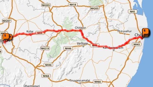
This illustrates how these parameters can be used to return the most appropriate hits for our scenario. Note that the figures only show the top hit for each query:

1. Searching for restaurants with the DistanceToPath feature. distance = 1000, traveled = 0.1
2. Searching for gas stations with the DistanceToPath feature. distance = 1000, traveled = 0.9